Welcome to RQL's Blog!

Do Better Every Day!

全球大气再分析资料

2022-06-21

renql

数据资料

CRA40
- CFSR
- JRA55
- MERRA2
- ERA5
- CRA40
- 参考文献
目前国际上使用的大气再分析资料已经历了多次迭代，除了以往被人们所熟知的NCEP1、NCEP2、ERA-interim，现在又出现了以下几个高分辨率的新品种（按发布顺序）。

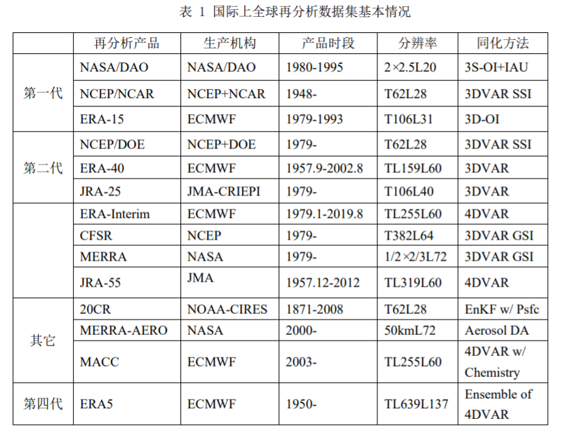
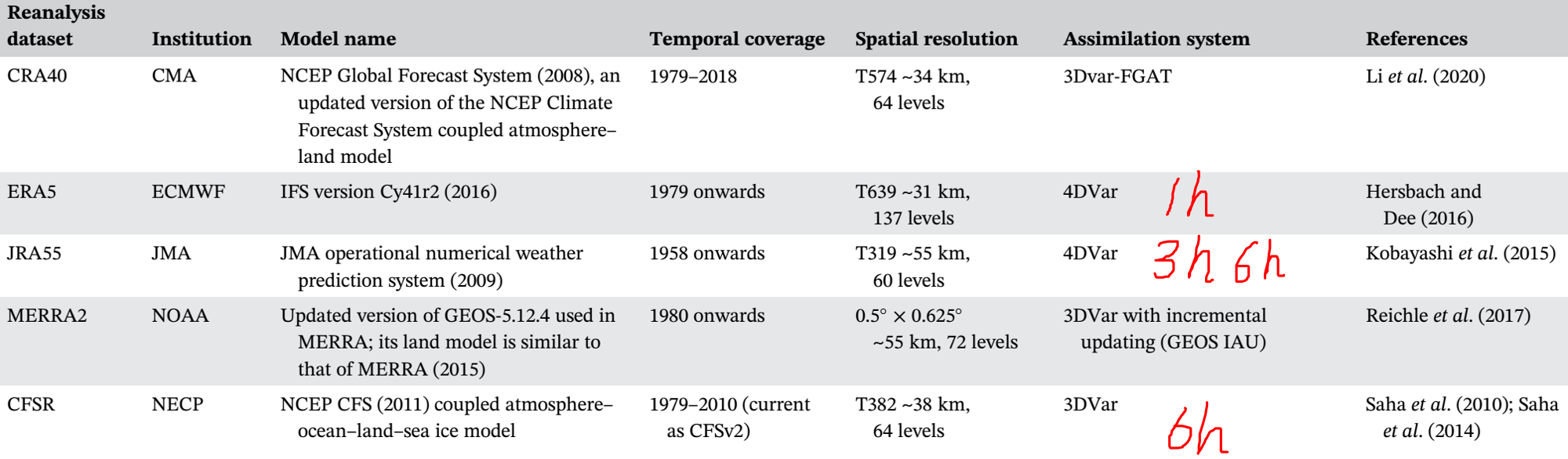
CFSR

NCEP（National Center for Environmental Prediction）于2010年发布的第3代全球再分析资料，全称Climate Forecast System Reanalysis，使用Coupled Forecast System (CFS) model，a coupled atmosphere–ocean–sea ice–land model, assimilates conventional observations and satellite radiance, and includes the time evolution of CO2 concentrations. 空间分辨率T382，约38km，垂直64层，使用GSI 3DVAR同化方法。

逐6h数据下载：https://rda.ucar.edu/datasets/ds093.0/#!description

JRA55

日本气象厅（Japanese Meteorological Agency）2013年发布的第二代再分析数据，基于全球谱模式JMA2002，水平分辨率T319（差不多0.5°分辨率），垂直60层，4D-Var semi-Lagrangian assimilation schemes with Variational Bias Correction (VarBC) for satellite radiances，采用新的辐射方案，引入随时间变化的温室气体浓度。有逐3h，逐6h。

数据下载地址：https://rda.ucar.edu/datasets/ds628.0/
日本气象厅的官网介绍：https://jra.kishou.go.jp/JRA-55/index_en.html

MERRA2

Modern-Era Retrospective analysis for Research and Applications, version 2 (MERRA-2)由 National Aeronautics and Space Administration (NASA) Global Modeling and Assimilation Office (GMAO)于2015年发布，基于Goddard Earth Observing System Model, Version 5 (GEOS-5) data assimilation system，时间跨度为1980至现在，分辨率 0.5lat x 0.625lon，垂直72层，有逐小时，逐3h，逐6h。

存在的缺陷：极低海域降水太大，热带区域山地降水偏多

数据官网介绍： https://gmao.gsfc.nasa.gov/reanalysis/MERRA-2/data_access/

ERA5

欧洲中期天气预报中心（European Centre for Medium-range Weather Forecasts，ECMWF）于2020年发布的、逐小时、31km水平分辨率的第五代再分析资料

CRA40

我国国家气象信息中心于2021年5月发布的、逐6小时、 34km水平分辨率的我国第一代全球大气和陆面再分析产品（CRA），下载网址 https://data.cma.cn/data/cdcdetail/dataCode/NAFP_CRA40_FTM_6HOR.html，但感觉下载不是很方便，需要注册一个国家气象科学数据中心的教育科研实名注册用户（需要上传省部级以上的科研项目书）。但气象局内部的人下载可能会方便一些。

我国的该项目启动于2014年，历时6年研制。基于Global System Model (GSM) of the Global Forecast System (GFS) of NCEP and its Gridpoint Statistical Interpolation (GSI) 3DVAR data assimilation system，同化了多种传统观测和卫星观测数据，尤其是东亚。

根据使用过的人反馈，质量比NCEP1好。但和ERA5及JRA55没有做过详细对比。

参考文献
- Li, C., T. Zhao, C. Shi, and Z. Liu, 2021: Assessment of precipitation from the CRA40 dataset and new generation reanalysis datasets in the global domain. Int. J. Climatol., 41, 5243–5263.
- Yu, X., L. Zhang, T. Zhou, and J. Liu, 2021: The Asian subtropical westerly jet stream in CRA-40, ERA5, and CFSR reanalysis data: Comparative assessment. J. Meteorol. Res., 35, 46–63.
Read All

python的主要结构

2022-03-12

renql

python

python数据结构
python输入输出
python运算
python的条件判断语句
几种python的循环语句
python 自定义函数
python读取nc文件

python数据结构

Python有五个标准的数据类型：Numbers（数字），String（字符串），List（列表），Tuple（元组），Dictionary（字典）

# 列表是写在方括号 [] 之间、用逗号分隔开的元素列表
list = [ 'abcd', 786 , 2.23, [1,2,3]]
tinylist = [123, 'runoob']
list2 = [i for i in range(30) if i % 3 == 0]
# 得到列表 [0, 3, 6, 9, 12, 15, 18, 21, 24, 27]

names = ['Bob','Tom','alice','Jerry','Wendy','Smith']
new_names = [name.upper()for name in names if len(name)>3]
# 得到列表 ['ALICE', 'JERRY', 'WENDY', 'SMITH']

print (len(list))       # 列表元素个数
print (list[3][0])      # 嵌套列表索引
print (list[1:3])       # 从第二个开始输出到第三个元素
print (list[2:])        # 输出从第三个元素开始的所有元素
print (list[-1::-1])    # 翻转列表
print (tinylist * 2)    # 输出两次列表
print (list + tinylist) # 连接列表

元组与列表类似，但元组的元素不能修改。
元组写在小括号 () 里，元素之间用逗号隔开
元组的索引及切片方式同list

# 字典用 {} 标识，它是一个无序的 键(key) : 值(value) 的集合
# 同一个字典中，键(key)必须是唯一且不可变的，因此数字，字符串或元组都可作为键，但列表不行。
dict1 = {}
dict1['one'] = "1 - 菜鸟教程"
dict1[2]     = "2 - 菜鸟工具"

tinydict = {'name': 'runoob','code':1, 'site': 'www.runoob.com'}

dict2 = {x: x**2 for x in (2, 4, 6)} 
# 得到的字典为{2: 4, 4: 16, 6: 36}

print (len(dict2))        # 计算字典元素个数，即键的总数。
print (dict['one'])       # 输出键为 'one' 的值
print (tinydict.keys())   # 输出所有键
print (tinydict.values()) # 输出所有值
del tinydict['Name'] # 删除键 'Name'
tinydict.clear()     # 清空字典

python输入输出

python列表和元组顺序也是从0开始的

a=input("please input password")
print("password you input is ",password)
print(type(a)) # input variable is usually str

b=int(a)
print(type(b))  

a=2
b='casename'
print('%s month is %03d'%(b,a))
# 格式化输出结果：casename month is 002

python运算

python中除号用/表示，但是和C语言不同的是/得到的值总是浮点数，例如：5 / 5结果是1.0。 python中整除用//表示是，//表示两数相除，向下取整，例如8 // 5 结果是1,，至于数据类型是整数还是浮点数则取决于用到的数据类型。

python的条件判断语句

不管是条件语句还是循环，命令最后都有冒号。

if a == 0 and b != 14:
	b = b+a
elif not a <= -1:
	b = b-a
else:
	b = b*a
	
list1 = ['a','b','coin']
if 'a' in list1:
	print('you are right')
	

几种python的循环语句

for i in range(-1,-10,-4):  
	print("Number of cycles: %d"%i)  
# 输出结果：
# Number of cycles: -1
# Number of cycles: -5
# Number of cycles: -9

name = 'chengdu'  
for i in name:
	print(i,end='\t') 
# '\t'是转义字符，表示水平制表符，即 Tab 键，一般相当于四个空格
# 输出结果：c	h	 e	n	 g	d	 u

b = [np.arange(d-lagh,d+lagh+1) for d in range(2,10,3)]
# 列表生成式

coins = ["Bitcoin", "Ethereum", "Cardano"]
prices = [48000,2585,2]
for coin, price in zip(coins, prices):
    print(f"${price} for 1 {coin}")

for i, coin in enumerate(coins):
    price = prices[i]
    print(f"${price} for 1 {coin}")

i = 0
while i < 5 :
	print('cycle time now : %d, i = %d'%(i+1,i))
	i += 1
else : 
	print('cycle end, now i = %d'%i)

break语句跳出 for 和 while 的循环体
continue 跳过当前循环，直接进行下一轮循环
pass 是空语句，一般用作占位语句，不做任何事情

python 自定义函数

除了正常定义的位置参数（也就是必选参数）外，还可以使用默认参数、可变参数（传入的参数个数可变）和关键字参数，使得函数定义出来的接口，不但能处理复杂的参数，还可以简化调用者的代码。

https://www.liaoxuefeng.com/wiki/1016959663602400/1017261630425888

python读取nc文件

import netCDF4 as nc   
f=nc.Dataset("/home/users/qd201969/ERA5-1HR/stat_apr-sep1979-2019.nc") # best to use absolute path  
f.variables.keys() # get the list of the variables   

a=f.variables['mstr'] # get the data and vari info  
a=f.variables['mstr'][:] # only get the data  
lat=f.variables['latitude'][:]  
lon=f.variables['longitude'][:]

indx=np.argwhere((lon<100) & (lon>10))
indy=np.argwhere((lat<50) & (lat>10))   

从xarray走向netCDF处理: https://www.jianshu.com/p/86f02bc58265

import xarray as xr
f = xr.open_dataset('EC-Interim_monthly_2018.nc') 

a=f['mstr'] # get the data and vari info
a=f.mstr    # two method to read the variable

b=a.loc[84.86:90,352.5:360] # use lat and lon read data
c=b.mean(dim=['lon','lat'])  

Read All

cdo常用命令

2022-03-08

renql

linux

数据

数据转换
数据合并
数据提取
数学运算
数据信息查看

CDO, climate data operator的缩写。提供了600多个常见的操作，能快速处理nc、grid等常见数据.

常见的功能包括：

数据的提取合并(提取特定时间、空间、经纬度等等)
数据的简单运算(加减乘除、方差、均方差、和、最值、滑动均值、滑动方差、滑动最值、区域平均、区域方差、区域最值等等)
数据的统计运算(相关、线性回归、EOF、滤波、水平插值、垂直插值等等)
数据的转换(binary转nc、HDF转nc等等)
各种气候指数的运算(极端有关的指数等等)

参考：https://blog.sciencenet.cn/blog-1081898-1275862.html

数据转换

转换数据类型或者转换文件类型

cdo -b F64 copy input.nc output.nc
# 将input.nc文件中的变量转换为 double，并另存为output.nc。如果不加F，则是将所有变量转换为double。加F则只是将floating data转为double

cdo -f nc copy input.grib output.nc
# 将grib文件转换为nc文件

数据合并

cdo -r -copy ff_stat_[1-9].nc ff_stat_1[0-2].nc outfilename
# 每月数据放在一个文件中，将1-12月共12个文件合并，-r表示合并后添加时间维，拼接后原始文件依然存在

cdo -cat uwind.1985-07.daily.nc uwind.1985-08.daily.nc outfilename
# 将两个文件中的变量按原有的时间维拼接，拼接后，原始文件依然存在
# 当输入文件过大且变量为short变量时，容易产生报错，解决方法是改用以下的代码，将short变量转换为float，-mergetime的作用等同于-cat
cdo -b F32 -mergetime ERA5_precip_1980-[1-9].nc ERA5_precip_1980-1[0-2].nc ERA5_precip_1hr_dec-jan1980.nc

数据提取

cdo selmonth,1 ERA5_NH_z_1981.nc ERA5_NH_z_1981-01.nc
# 提取一个月的数据，注意选项与参数间的逗号

cdo sellevel,850 ERA5_NH_z_1981.nc ERA5_NH_850z_1981.nc
# 提取某个高度的数据，注意选项与参数间的逗号

数学运算

cdo expr,’speed=sqrt(sqr(uwnd)+sqr(vwnd));var2=ts-273.15;’ infile outfile
# infile中有变量uwnd，vwnd，ts。由这三个变量计算新变量并存储入 outfile

数据信息查看

除了处理数据外，cdo也能快速查看 grid、nc 等数据文件信息，常用参数有：

cdo sinfon ERA5_wind10_2016.grib #输出数据文件的简短信息

参考自：https://cloud.tencent.com/developer/article/1618318

Read All

Xarray用法

2022-03-02

renql

python

xarray

DataArray数组创建
Dataset数组创建
indexing, isin and groupby
读取多个nc文件
读取grib数据
Masking
apply_ufunc批量处理多维数组

dimension:维度
coordinate：坐标
一个维度可以被赋予多个坐标，因此一般坐标数量多于纬度数

DataArray数组创建

data = np.random.rand(4, 3)
locs = ["IA", "IL", "IN"]
times = pd.date_range("2000-01-01", periods=4)
foo = xr.DataArray(data, coords=[times, locs], dims=["time", "space"])
foo = xr.DataArray(data, coords=[("time", times), ("space", locs)])
foo.attrs['units']='mm/day' # 修改或创建数据属性参数
del foo.attrs['projection'] # 删去某个属性
foo.drop('time',dim=None) # 删去time维对应的坐标，但保留维度
foo.rename({'dayofyear':'time'}) # 修改某个纬度的名字
foo.coords['time'] = times # 修改某个维度的坐标

foo.dtype # dtype('float32')
foo.dims # ('time', 'space')
var.shape # (10248, 1, 256, 512)
var.min()

Dataset数组创建

temp = 15 + 8 * np.random.randn(2, 2, 3)
precip = 10 * np.random.rand(2, 2, 3)
lon = [[-99.83, -99.32], [-99.79, -99.23]]
lat = [[42.25, 42.21], [42.63, 42.59]]
ds = xr.Dataset(
	{
	       "temperature": (["x", "y", "time"], temp),
               "precipitation": (["x", "y", "time"], precip),
	},
	coords={
		"lon": (["x", "y"], lon),
                "lat": (["x", "y"], lat),
                "time": pd.date_range("2014-09-06", periods=3),
                "reference_time": pd.Timestamp("2014-09-05"),
	},
)

# Dictionary like methods to update a dataset 
ds = xr.Dataset()
ds["temperature"] = (("x", "y", "time"), temp)
ds["temperature_double"] = (("x", "y", "time"), temp * 2)
ds["precipitation"] = (("x", "y", "time"), precip)
ds.coords["lat"] = (("x", "y"), lat)
ds.coords["lon"] = (("x", "y"), lon)
ds.coords["time"] = pd.date_range("2014-09-06", periods=3)
ds.coords["reference_time"] = pd.Timestamp("2014-09-05")

ds = da.to_dataset(name="temp") #将da这个DataArray加入到ds这个数据组中，并命名为 temp
ds.to_netcdf(fileout+varname+".nc","w") #存储ds文件

# the use of pipe
plt.plot((2 * ds.temperature.sel(x=0)).mean("y"))
(ds.temperature.sel(x=0).pipe(lambda x: 2 * x).mean("y").pipe(plt.plot))

To remove a dimension or a variable, you can use below method, which will return a new dataset. Any variables using that dimension are dropped:

ds_new = ds.drop_vars("temperature")
ds_new = ds.drop_dims("time")

ds_new.coords['month']=range(1,13,1) # add a new dimension

indexing, isin and groupby

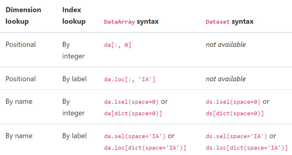
import xarray as xr
import numpy as np
lonl=0  
lonr=150
lats=15 
latn=70

ds  = xr.open_dataset("ERA5_precip_1hr_dec-jan1989.nc")
lat = ds.latitude
lon = ds.longitude
ilon = lon[(lon>=lonl) & (lon<=lonr)]
ilat = lat[(lat>=lats) & (lat<=latn)]
term = ds['tp'][0,:,:]
term = ds['tp'].sel(time=ds.time.dt.year.isin(1989),longitude=ilon,latitude=ilat)
# <xarray.DataArray 'tp' (time: 8760, latitude: 221, longitude: 601)>
term.mean(('latitude','latitude'))

term.sel(time=slice("2000-01-01", "2000-01-02"))
var = term.sel(time=term.time.dt.month.isin(1)).mean("time")
term.loc[ct,:,:] = term.sel(time=ct).mean('time')
# loc是定位，sel是截取部分变量

# calculate monthly data
var = term.groupby(term.time.dt.month)
# DataArrayGroupBy, grouped over 'month'
# 12 groups with labels 1, 2, 3, 4, 5, 6, 7, 8, 9, 10, 11, 12.
print(var.sum("time"))
# <xarray.DataArray 'tp' (month: 12, latitude: 221, longitude: 601)>

ds1=ds.groupby(ds.time.dt.month).mean('time')
ds1=ds.groupby('time.month').mean('time')
ds1=da.groupby('time.dayofyear').mean('time') # 365天
ds_weighted = (ds * weights).groupby('time.season').sum(dim='time') # 'DJF' 'JJA' 'MAM' 'SON'

读取多个nc文件

fs = xr.open_mfdataset(file_string, combine='nested', concat_dim='time', parallel=True) 
# file_string 可以是一个字符串“path/to/my/files/*.nc”，也可以是文件路径列表  
# combine 有两种选项 "by_coords" 和 "nested"
# concat_dim 表示将文件沿某一维度连接，只有 combine='nested' 时需要提供这一选项。
# 若concat_dim是已存在的维度，则文件沿该维度连接，若concat_dim是不存在的维度，则文件沿新的维度连接

var = fs['temp'].data
term=[var[i:i+3,:,:].sum(axis=0) for i in range(0,25587,3)] # 得到一个list
var1 = np.array(term).reshape(8529*nlat*nlon) #转成一维数组

读取grib数据

主要依赖的库是 https://pypi.org/project/cfgrib/ ，该库可以把grib文件投影到netcdf格式。
可以搭配xarray使用，使用方法如下。可以一次读取一个文件，也可以用xr.open_mfdataset读取多个文件，其他用法同netcdf

ds = xr.open_dataset('example.grib', engine='cfgrib')
print(ds)

# 目前cfgrib库无法同时读取多个typeOfLevel，因此需要根据提示筛选我们需要的数据。
# 这个typeOfLevel可以是isobaricInhPa，surface，depth_below_land  
ds = xr.open_dataset('example.grib2', engine="cfgrib", backend_kwargs={'filter_by_keys': {'typeOfLevel': 'isobaricInhPa'}})
print(ds)

默认情景下，cfgrib会输出一个index文档（后缀为.idx），该索引文档可随时删除它们，并在出现问题时重试。当grib文件所处目录不支持写入文件时，即cfgrib无法在该目录下保存索引文档，此时便会出现如下报错信息，但该报错信息不影响grib数据的读取。也可在backend_kwargs中加入’indexpath’:’‘选项来选择不输出该索引文档，此时上述报错信息便会消失。

Can't create file '/home/metctm1/array_hq133/data/drv_fld/era5/20220803-sl.grib.923a8.idx'
Traceback (most recent call last):
  File "/home/metctm1/array/soft/anaconda3/lib/python3.8/site-packages/cfgrib/messages.py", line 343, in from_indexpath_or_filestream
    with compat_create_exclusive(indexpath) as new_index_file:
  File "/home/metctm1/array/soft/anaconda3/lib/python3.8/contextlib.py", line 113, in __enter__
    return next(self.gen)
  File "/home/metctm1/array/soft/anaconda3/lib/python3.8/site-packages/cfgrib/messages.py", line 264, in compat_create_exclusive
    fd = os.open(path, os.O_WRONLY | os.O_CREAT | os.O_EXCL)
PermissionError: [Errno 13] Permission denied: '/home/metctm1/array_hq133/data/drv_fld/era5/20220803-sl.grib.923a8.idx'
Can't read index file '/home/metctm1/array_hq133/data/drv_fld/era5/20220803-sl.grib.923a8.idx'
Traceback (most recent call last):
  File "/home/metctm1/array/soft/anaconda3/lib/python3.8/site-packages/cfgrib/messages.py", line 353, in from_indexpath_or_filestream
    index_mtime = os.path.getmtime(indexpath)
  File "/home/metctm1/array/soft/anaconda3/lib/python3.8/genericpath.py", line 55, in getmtime
    return os.stat(filename).st_mtime
FileNotFoundError: [Errno 2] No such file or directory: '/home/metctm1/array_hq133/data/drv_fld/era5/20220803-sl.grib.923a8.idx'

若要循环处理多个文件，可以先利用list来存储数据，然后再转成numpy进行数学运算

    var = []
    fn_stream = subprocess.check_output(
        'ls %s/%d07*-%s.grib'%(
        indir[0],year,suffix), shell=True).decode('utf-8')
    fn_list = fn_stream.split()

    for itm in fn_list:
        ds = xr.open_dataset(itm,engine='cfgrib',backend_kwargs={
                'filter_by_keys': {'typeOfLevel': 'surface'}})
        var.append(ds[varname].data.tolist())
	
    var = np.array(var).mean(axis=0)

Masking

da = xr.DataArray(np.arange(16).reshape(4, 4), dims=["x", "y"])
da.where(da.x + da.y < 4)
# 保留满足条件的变量，未满足条件的变量设为nan
# da.where(da.x + da.y < 4，0)，会将未满足条件的变量设为0

# output is 
# <xarray.DataArray (x: 4, y: 4)>
# array([[ 0.,  1.,  2.,  3.],
#        [ 4.,  5.,  6., nan],
#        [ 8.,  9., nan, nan],
#        [12., nan, nan, nan]])
# Dimensions without coordinates: x, y

da = xr.DataArray([1, 2, 3, 4, 5], dims=["x"])
lookup = xr.DataArray([-1, -2, -3, -4, -5], dims=["x"])
da.where(lookup.isin([-2, -4]), drop=True) # output array([2., 4.]) 
# 加 drop=True后，未满足条件的变量会被删去，数据结构发生变化
# when done repeatedly, this type of indexing is significantly slower than using sel().

apply_ufunc批量处理多维数组

from scipy import stats
def new_linregress(x, y):
    # Wrapper around scipy linregress to use in apply_ufunc
    slope, intercept, r_value, p_value, std_err = stats.linregress(x, y)
    return np.array([slope, p_value])

a1 = xr.apply_ufunc(new_linregress, t, t,
                       input_core_dims=[['time'], ['time']],
                       output_core_dims=[["parameter"]],
                       vectorize=True,
                       dask="parallelized",
                       output_dtypes=['float64'],
                      )
# dimension of t is (time: 10248, lat: 3, lon: 4)
# a1 is (lat: 3, lon: 4, parameter: 2)

ts=np.zeros([2,3,10248],dtype=float)
locs = ['EA','NA']
month = ['DJF','MAM','JJA']
ts1 = xr.DataArray(ts, coords=[locs,month,t.time], dims=["space","month","time"])

a1 = xr.apply_ufunc(new_linregress, t, ts1,
                       input_core_dims=[['time'], ['time']],
                       output_core_dims=[["parameter"]],
                       vectorize=True,
                       dask="parallelized",
                       output_dtypes=['float64'],
                      )
# a1 is (lat: 3, lon: 4, space: 2, month: 3, parameter: 2)

Read All

英语论文写作常用句式

2022-01-09

renql

English_learning

学术论文
- 文章标题
- Abstract
  - 摘要第一句话
绝热与非绝热经常搞混的几个单词： diabatic 非绝热的，传热的 adiabatic 绝热的，不传热的 adiabatically

文章标题
- climate changes in sth/ (over sp) 什么的气候变化
- climate effects of sth 什么的气候效应
- response of sth to sth
- Seasonally-dependent impact of easterly wind bursts on the development of El Niño events
- Role of Atlantic air–sea interaction in modulating the effect of Tibetan Plateau heating on the upstream climate over Afro-Eurasia–Atlantic regions
- Signals of Spring Thermal Contrast Related to the Interannual Variations in the Onset of the South China Sea Summer Monsoon
- Multi-scale temporal-spatial variability of the East Asian summer monsoon frontal system: observation versus its representation in the GFDL HiRAM
- Sources of Subseasonal Prediction Skill for Heatwaves over the Yangtze River Basin Revealed from Three S2S Models
Abstract

摘要第一句话
- The location change of the westerly jet core at upper troposphere in June and July is investigated by using the NCEP/NCAR reanalysis data.
- In this study, 40-yr ECMWF Re-Analysis (ERA-40) data are used for the description of the seasonal cycle and the interannual variability of the westerly jet in the Tibetan Plateau region.
- This study examines the representation of the multi-scale temporospatial variability of the East Asian summer monsoon stationary front (MSF) in the High-Resolution Atmospheric Model (HiRAM) of the National Oceanic and Atmospheric Administration (NOAA) Geophysical Fluid Dynamics Laboratory.
- The structure and dynamics of decadal anomalies in the wintertime midlatitude North Pacifc ocean–atmosphere system are examined in this study, using the NCEP/NCAR atmospheric reanalysis, HadISST SST and Simple Ocean Data Assimilation data for 1960–2010.
- It is suggested that the midlatitude ocean–atmosphere interaction can provide a positive feedback mechanism for the development of initial anomaly, in which the oceanic front and the atmospheric transient eddy are the indispensable ingredients.
- Such a positive ocean–atmosphere feedback mechanism is fundamentally responsible for the observed decadal anomalies in the midlatitude North Pacific ocean–atmosphere system.
Read All
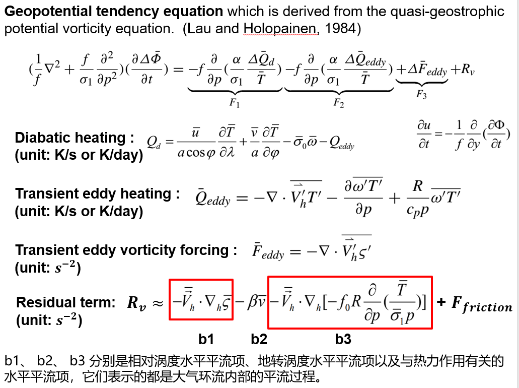
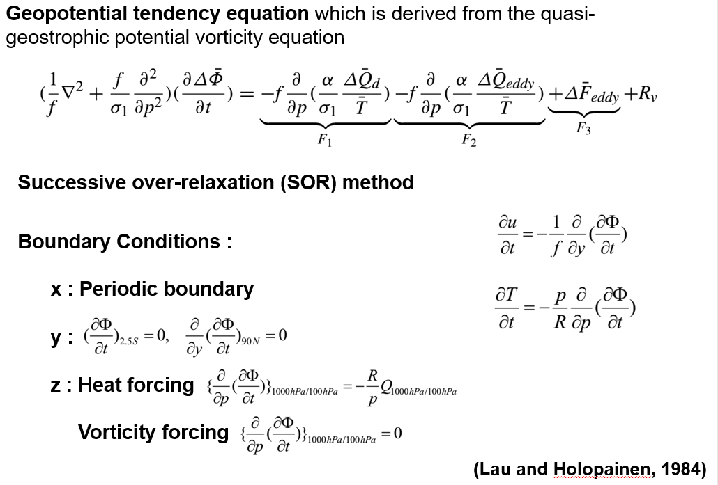
位势倾向方程

2022-01-01

renql

大气科学

诊断量
总体特征与用途

瞬变涡旋对气候态的影响在大气环流的理论和观测研究中都是一个基本问题。TE可以通过重新分配热量和涡度影响大气状态。因此TE对气候态的平衡可以用TE通量的辐合辐散表示。

但是，静力平衡和准地转约束要求TE通量的产生必须伴随次级环流，而这又会影响气候态。因此若要全面理解TE对平均流的净效应，除了要考虑TE通量的辐合辐散外，也要考虑由TE引起的环流的影响。

以往的研究通过假设TE通量的辐合辐散为热量和涡度的源汇，通过求解方程，计算出定常响应，来解决上述问题。这些研究表明TE会减弱由地形强迫出来的定常波的振幅。但这些耗散效应的定量估计对模式假设非常敏感。

除了寻找时间平均方程的有限振幅解外，也可以通过考察当加入TE强迫时的瞬时初始大气响应。且最好用准地转系统来研究这个问题，这可以保证计算结果满足静力平衡及地转平衡。如果用原始方程来研究这个问题，会获得一个有很多不真实小扰动的初始倾向。

因此Lau于1984年利用时间平均的准地转位涡方程，通过设定合适的边界条件（其中热力强迫项的边界条件根据静力平衡和时间平均温度公式推导得到），求解出由TE驱动出来的三维分布的准地转位势倾向，然后根据地转风关系和静力平衡求解地转风倾向及温度倾向。这些初始倾向满足静力平衡及地转平衡，因此可以将由eddy引起的环流和TE通量散度同时考虑进去。

由于Lau1984年的文章只考虑了准地转大气对TE强迫的响应，因此可以将平流项和摩擦项等忽略。

反算泊松算子求解位势倾向时，Lau1984用的是球谐波函数差分迭代（我也不太懂），而现在多用超松弛迭代法。

缺点：
1. 强迫对局地环流的影响最大，随距离增大，强迫影响减弱。因此在局地强迫强的情况下，主要体现局地强迫的作用，难以查看遥相关的作用。或许相关回归可以。
2. 计算得到的气候态结果（尤其热力强迫项驱动的位势倾向）对上下边界条件敏感，但若看其回归场之类的结果还可以。
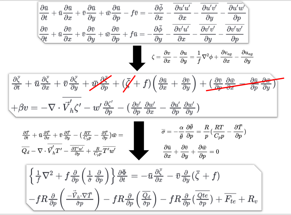
方程及推导过程

\begin{split} \bar \sigma_0 = \frac{R}{C_p} \frac{\bar T}{p} - \frac{\partial \bar T}{\partial p} \\
\bar \sigma_1 = \frac{R \bar \sigma_0}{p} \end{split}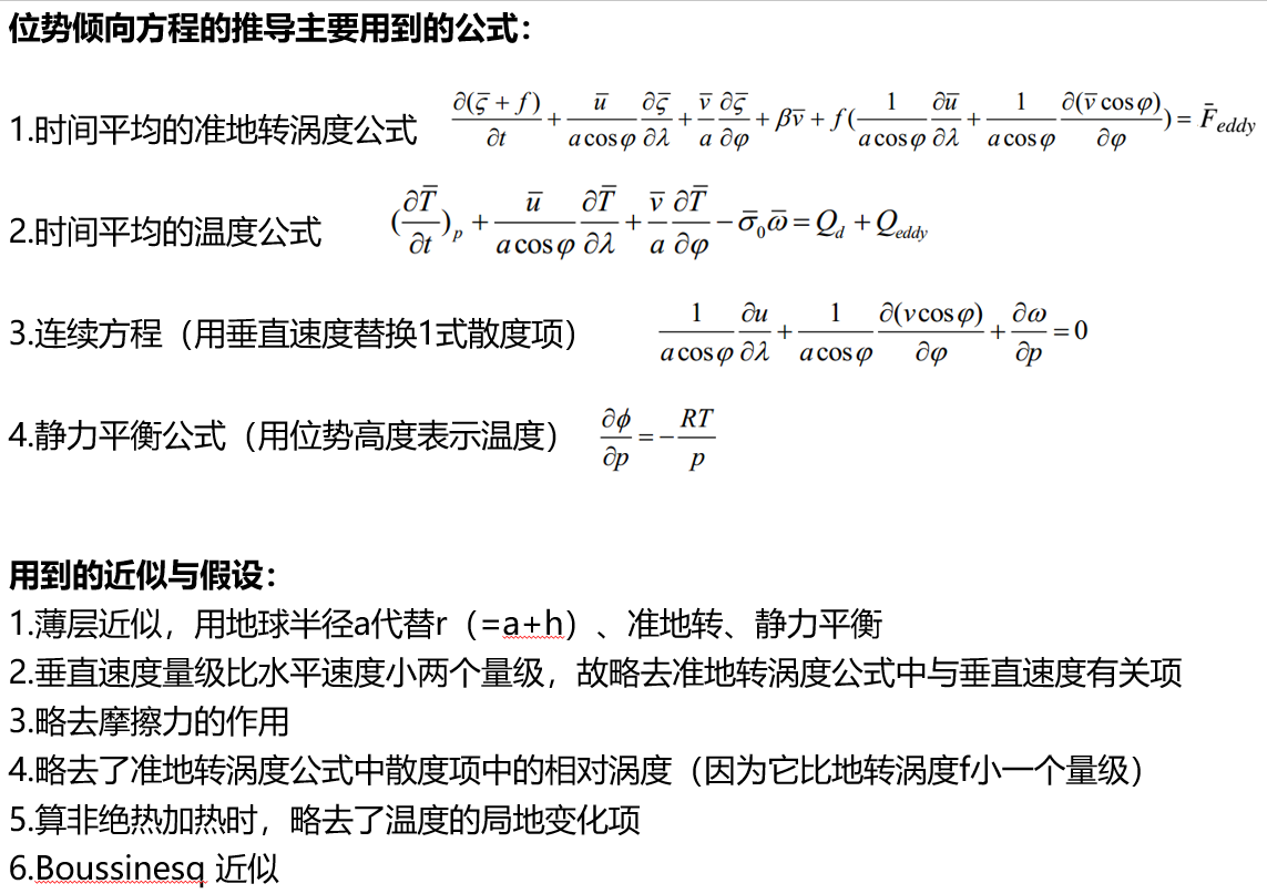

计算结果

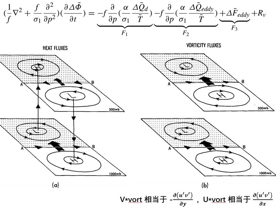
迭代计算位势倾向时，由于热力项的垂直边界条件和瞬变涡旋强迫的不同，导致其计算结果也不同。理想情况下的解析解情况：
1. 当F2为负且随高度不变时，但上下边界依旧不同.此时对应的情况有两种：当eddy热量辐合（为正，加热）随高度线性减弱至0，因此上边界条件为0，下边界条件为负，此时得到底层为负的位势倾向，即产生底层低气压气旋，高层倾向于产生高气压反气旋，具有斜压性。若是eddy热量辐散（为负，冷却）随高度增加，上边界为正，下边界为0，F2为负，结果与之相同。
2. 当F3为负且随高度不变时，即eddy涡度通量辐散整层均一，那么整层都产生相同正位势倾向，即产生高气压反气旋。准地转纬向风倾向垂直于eddy涡度通量并指向其右方。
一般在风暴轴处伴随有向极的eddy热量通量和eddy涡度通量。而这向极的eddy热量通量，会增强上层东风，增强下层西风。向极的eddy涡度通量则会增强整层的西风。因此eddy热量通量和eddy涡度通量对纬向风的作用在底层一样（增强西风），高空则相反。

计算时可能遇到的问题
1. 使用迭代方法时，不能存在缺测，可将缺测的UVTW进行纬向插值或径向插值。
2. 由于热力强迫项的结果对上下边界条件敏感，而对于地形复杂的地方，底层数据存在较多缺测。因此，一般在选择原始数据时，底层数据层数尽量少选。同时用准地转关系替换1000、925hPa的风场，最后用log插值（Lau1984用的时三次样条插值，我个人感觉几种插值方法结果差不多）的方法把15层（1000, 925, 850, 700, 600, 500, 400, 350, 300, 250, 200, 175, 150, 125, 100）数据插到21层（1000, 950, 900, 850, 800, 750, 700, 650, 600, 550, 500, 450, 400, 350, 300, 250, 200, 175, 150, 125, 100）
3. 计算非绝热加热时，$\sigma_0$不需要取半球平均。但在求F1和F2时，静力稳定度$\sigma_1$需要取半球平均或时间平均，否则会因为底层的静力稳定度趋向于0，导致底层非绝热加热的垂直梯度异常大，影响计算结果。同时在迭代过程中，迭代系数中的静力稳定度也需要取半球平均，否则迭代无法收敛。此处，静力稳定度之所以可以取半球平均，是因为其水平均一只随高度变化，这是准地转下适用的假设。另外，基于热带的层结稳定度与中高纬度间存在较大差异，所以静力稳定度最好取20N以北的区域平均。不过冬天以及气候平均态的情况下，应该影响不大。
4. 在计算强迫项和迭代系数时，是否固定科式参数会对低纬地区的解存在一定影响。从10N度开始迭代，需要固定科式参数，热力强迫出的位势倾向才会具有斜压结构。但若从15N度开始迭代，不固定科式参数也能出现斜压结构。目前来看，还是尽量不要固定科式参数。
参考文献
1. Lau, N. C., and E. O. Holopainen, 1984: Transient eddy forcing of the time-mean flow as identified by geopotential tendencies. J. Atmos. Sci., https://doi.org/10.1175/1520-0469(1984)041<0313:TEFOTT>2.0.CO;2.
2. Fang, J., and X. Q. Yang, 2016: Structure and dynamics of decadal anomalies in the wintertime midlatitude North Pacific ocean–atmosphere system. Clim. Dyn., https://doi.org/10.1007/s00382-015-2946-x.
3. 李蕊. 瞬变强迫在北半球冬季环状模变异中的作用[D].南京大学,2013.
4. Ren, Q., X. Jiang, Y. Zhang, Z. Li, and S. Yang, 2021: Effects of Suppressed Transient Eddies by the Tibetan Plateau on the East Asian Summer Monsoon. J. Climate, https://doi.org/10.1175/jcli-d-20-0646.1. 用位势倾向方程诊断东亚夏季的气候态环流变化原因
5. Ren, Q., W. Wei, M. Lu, and S. Yang, 2022: Dynamical analysis of the winter Middle East jet stream and comparison with the East Asian and North American jet streams. J. Climate, accepted. 用位势倾向方程诊断东亚急流、中东急流、北美急流的物理维持过程并对比
Read All

2/23

Principle

Welcome to RQL's Blog!

全球大气再分析资料

CFSR

JRA55

MERRA2

ERA5

CRA40

参考文献

python的主要结构

python数据结构

python输入输出

python运算

python的条件判断语句

几种python的循环语句

python 自定义函数

python读取nc文件

cdo常用命令

数据转换

数据合并

数据提取

数学运算

数据信息查看

Xarray用法

DataArray数组创建

Dataset数组创建

indexing, isin and groupby

读取多个nc文件

读取grib数据

Masking

apply_ufunc批量处理多维数组

英语论文写作常用句式

文章标题

Abstract

摘要第一句话

位势倾向方程

总体特征与用途

方程及推导过程

计算结果

计算时可能遇到的问题

参考文献