一、散度涡度 divergence and vorticity

；以下是用中央差分的方法计算涡度散度
	divg = uv2dv_cfd ( uwnd, vwnd, uwnd&lat, uwnd&lon, scalar-integer )
	vort = uv2vr_cfd ( uwnd, vwnd, uwnd&lat, uwnd&lon, scalar-integer )
	;scalar-integer设为0，边界点都将设为缺测值；
	;1，则uwnd和vwnd在经度上刚好围城一个圆，此时设置上边界和下边界为缺测值；
	;2，边界点用单向差分法估计；
	;3，uwnd和vwnd在经度上刚好围成一个圈，无重复点，此时上边界和下边界分别用单向差分法估计。
	
；以下是用球谐函数 spherical harmonics 的方法计算涡度散度，  
；用球谐函数计算得到的散度和涡度比中央差分计算得到的值更精确。  
；但只有只有当输入的风场是全球风场且无缺测值时方可使用球谐函数计算。  
	uv2vrdvf ( uwnd, vwnd, vort, divg ) ;计算涡度和散度，括号中后两个值是返回值。  
	divg = uv2dvF_Wrap( uwnd, vwnd )
	vort = uv2vrF_Wrap( uwnd, vwnd )

虽然官网说用球谐函数计算散度和涡度比用中央差分法更精确，但我在用乳源地区的日降水量与涡度散度算相关时，却发现用球谐函数计算得到的散度和涡度不是很靠谱。

二、流函数和速度势计算

无辐散流有流函数，流函数的拉普拉斯是涡度，流函数的高值中心代表反气旋（顺时针），低值中心代表气旋（逆时针）
无旋转流有速度势，速度势的拉普拉斯是散度

uv2sfvpf ( uwnd, vwnd, stream_function, velocity_potential )  
;calculate stream function and velocity potential via spherical harmonics on a fixed grid
sfvp2uvf ( stream_function, velocity_potential, uwnd, vwnd )
;Computes the wind components given stream function and velocity potential (on a fixed grid) via spherical harmonics.

uv2vrf (uwnd,vwnd,vort)  ;calculate the vorticity via spherical harmonics on a fixed grid   
vr2uvf (vort,ur,vr)      ;calculate the rotational wind components via spherical harmonics on a fixed grid
;ur and vr are the return data 

uv2dvf (uwnd,vwnd,divg)  ;calculate the vorticity via spherical harmonics on a fixed grid   
dv2uvf (divg,ud,vd)      ;calculate the divergent wind components via spherical harmonics on a fixed grid
;ud and vd are the return data 

;the data used by these function must be on a global grid and no missing values    
;If any missing values are encountered in a particular 2D input grid, 
;then all of the values in the corresponding output grids will be set to the missing value
;if there are missing values, you can make the missing value zero by this method
uwnd = where(ismissing(uwnd),0,uwnd)

sf = sf/1000000    ;the stream function's unit is m^2/s, and the magnitude is large, so divided by 10^6
copy_VarMeta(vars,sf(0,0,:,:))

三、经圈质量流函数

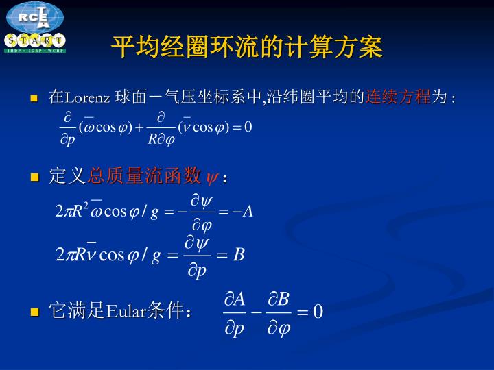
上图显示的是全球纬向平均的经圈质量流函数的推导过程，一般常用该流函数来研究Hadley环流。其具体计算方案及计算结果如下图所示。

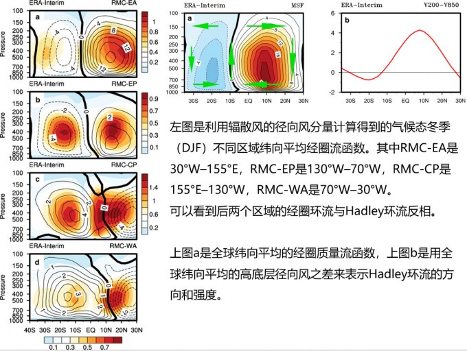
综上，研究Hadley环流的诊断量有以下三种：

利用径向风计算的全球纬向平均的经圈质量流函数，但它忽略了热带大气环流的区域多样性
The vertical shear of the meridional wind between 200 and 850 hPa (V200–V850)，可以用于研究Hadley环流强度的纬向变化，已有学者利用该诊断量研究Hadley环流的多尺度变率及其与其他气候现象（如ENSO）间的关系。但无法用该指数精确定义Hadley环流的南北边界
利用辐散风的径向风分量计算的区域纬向平均的经圈流函数，即可以研究Hadley环流的纬向变化，又可以确定Hadley环流的强度及南北范围。但该指数只用到了环流的辐散风分量，无法全面描述环流整体的变化。

此外，用经向风的辐散分量计算全球纬向平均经圈质量流函数同用原始经向风的计算结果。

参考文献：

Zhang, G. and Z. Wang, 2013: Interannual Variability of the Atlantic Hadley Circulation in Boreal Summer and Its Impacts on Tropical Cyclone Activity. J. Climate, 26, 8529–8544, https://doi.org/10.1175/JCLI-D-12-00802.1
Sun, Y., Li, L.Z.X., Ramstein, G. et al. 2019: Regional meridional cells governing the interannual variability of the Hadley circulation in boreal winter. Clim Dyn, 52: 831. https://doi.org/10.1007/s00382-018-4263-7
Nguyen, H., Hendon, H.H., Lim, E.P. et al. 2017: Variability of the extent of the Hadley circulation in the southern hemisphere: a regional perspective. Clim Dyn, 50: 129. https://doi.org/10.1007/s00382-017-3592-2

ncl计算方案大约有两种：

直接用ncl自带的函数计算 zonal_mpsi (v,lat,p,ps) ，但该函数只能计算经圈流函数，且若计算区域经圈环流，需先将径向风的辐散分量计算出来，再利用该函数。
自己做垂直积分计算。这样还可以用于计算纬圈流函数。
经检验，两种计算结果类似。

v   = new((/nlev,nlat,nlon/),float)
ps  = new((/nlev,nlat,nlon/),float)
msf = new((/nlev,nlat/),float)

;方案1
msf   = zonal_mpsi_Wrap(v(::-1,:,:),v&lat,plev(::-1)*100,ps)
msf_m = msf(::-1,:) 

;方案2
g  = 9.8 ;m/(s*s)
a  = 6378388 ;the radius of earth, m
pi = atan(1.0)*4
lat  = vars&lat
ptop = 0
iopt = 0
dp  := dpres_plevel(plev*100,ps,ptop,iopt)
dpm = dim_avg_n(dp,2)
v_m = dim_avg_n(v,2)
do inl = 0, unlev-1, 1
    msf_m(inl,:) = dim_sum_n(v_m(inl:nlev-1,:)*dpm(inl:nlev-1,:),0)
    msf_m(inl,:) = msf_m(inl,:)*2*pi*cos(lat*pi/180.0)*a/g
end do

msf_m = msf_m/10^10
copy_VarMeta(v(:,:,0),msf_m)

辐散风和旋转风

一、散度涡度 divergence and vorticity

二、流函数和速度势计算

三、经圈质量流函数